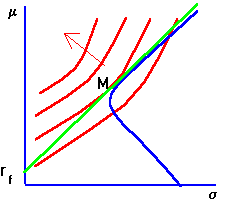
On-line, you can popup a window containing the above graph by clicking on risk-averse investor graph now.

As you move from left to right along a single indifference curve, both risk and expected return increase. That is, to provide this investor with the same level of expected utility requires that expected return increase to compensate for the additional risk. As you move in a northwest direction, shown by the arrow, the expected utility increases. This is because by moving in this direction you are increasing expected return and decreasing risk.

Once we have the indifference map, we can study the investor's portfolio choice. The investor is constrained by the available set of investment opportunities. The investment opportunity set for risky securities is represented by the set of points bounded by the set of minimum-variance portfolios.

Observe that the best a risk-averse investor can ever do is to select the point of tangency between an individual indifference curve and the capital market line (CML). This is because the CML is the locus of portfolios that dominate all other portfolios in terms of portfolio return and risk.

We have drawn Figure 7.4, (which can be displayed on-line by clicking on risk-averse investor graph) so that the investor's indifference map is tangent to the CML exactly at portfolio M. This is also the point of tangency between the CML and the (blue) minimum-variance frontier. That is, our investor exactly chooses portfolio M and does not borrow or lend at the risk-free rate.

In general, preferences are unlikely to be such that the point of tangency to the CML is exactly at M. That is, for more (less) risk-averse investors, the indifference maps will form points of tangency with the capital market line at other points along the CML.

Let us consider first what is meant by an investor being more or less risk-averse. If Investor A is more risk-averse than Investor B, the two will have differently shaped indifference curves. To stay at the same level of expected utility as we move along A's indifference curve, A will require more expected return to compensate for the additional risk than will B. As a result, A's indifference curve is more steeply sloped than B's indifference curve.

For example, consider the points of tangency between Investor A's indifference map at portfolio N and B's indifference map at portfolio P on the CML depicted in Figure 7.7.

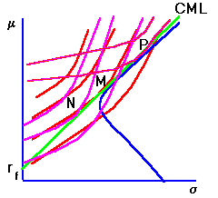
Investor A's indifference map has a steeper (negative) slope than does Investor B's indifference curve. Since N lies below portfolio M, Investor A chooses to invest some wealth in the risk-free asset and some wealth in the risky portfolio. This provides a higher expected utility point to Investor A than does his/her indifference curve that passes through point P on the capital market line.

This is because Investor A requires a lot more expected return in order to invest in the riskier position P, given the existing market price of risk. Investor B however, is less risk-averse than Investor A, and requires less expected return to assume additional risk. As a result, the indifference curve that passes through N provides Investor B with a lower level of expected utility than the indifference curve that passes through P. Investor B, therefore, increases expected utility by borrowing at the risk-free rate to purchase additional amounts of the market portfolio M.

The important point to note is that whatever their risk aversion, any investor will choose some combination of the risk-free asset and M. This forms the basis for an important

result called the two-fund theorem.

(C) Copyright 1999, OS Financial Trading System