6

6.11 Zero-Beta Portfolios

Now, we derive a general form of the SML. This relationship holds with or without a risk-free asset. We will obtain the result when there is no risk-free asset.

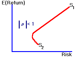
Recall that in the two-security problem with short selling, any combination of the two securities lies on the minimum variance frontier of risky assets.

Figure 6.5

Two-Security Frontier

Now, consider the same two-security problem where, in the place of two individual securities, we substitute two distinct mean variance efficient portfolios, say, P1 and P2. Suppose we form a third portfolio from these two efficient portfolios. That is, consider Portfolio P such that:

where

To establish that any portfolio of two mean variance efficient portfolios is itself an efficient portfolio (when short selling is allowed), we will demonstrate that the first-order conditions to the general minimum-variance problem with short selling (see Chapter 4, topic 4.6, N-Security Case), are satisfied by forming a portfolio from these two portfolios.

The portfolio weights in the two efficient portfolios are solutions to respective Lagrange problems where the first-order conditions are all linear and equal to zero. Consider the minimum-variance problem constructed from the weighted average of the two original Lagrange problems denoted as Problems 1 and 2 respectively. If the portfolio weights in Problem 1 are denoted by the vector a and the portfolio weights in Problem 2 denoted by the vector b then the weight in the combined portfolio of the two minimum-variance portfolios, for any security i, is:

Thus the first-order conditions in this combined problem are linear combinations of the linear first-order conditions of the two original Lagrange problems. Since these conditions in the two original problems equal zero, the first-order conditions in the combined problem will also equal zero. As a result, this combined portfolio is itself a minimum-variance portfolio.

Furthermore, since short selling is permitted, any target return can be constructed, and the entire efficient frontier of risky assets can be created from these two minimum-variance portfolios.

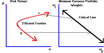
This result is a generalization of the result obtained from the geometric analysis of the three-security problem as in Figure 6.6. In Figure 6.6 two minimum-variance portfolios are fixed, I and II. A portfolio of I and II is formed by varying the weights on I and II respectively, wI, and wII, which traces out the critical line as shown.

Figure 6.6

Portfolio of Two Minimum-Variance Portfolios

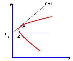
To derive the general form of the SML, we first fix an arbitrary minimum-variance portfolio and call it M. With unlimited short selling, we can find another portfolio that has a zero covariance with M, called Z.

Geometrically, Portfolio Z can be obtained by drawing a horizontal line from the intersection with the return axis, of the line whose point of tangency is M, to the intersection of the efficient frontier of risky assets. This point Z is depicted in Figure 6.7.

Figure 6.7

Zero Covariance Portfolio Pair

Graphically, a new CML is constructed from the risk/return characteristics of portfolios M and Z.

The risk/return characteristics for portfolios that lie on this new CML are:

and because M and Z have zero covariance, the portfolio risk equals:

Finally, the efficient set mathematics implies the same linear risk/return relationship for each security as described by the security market line (SML). However, in the present case the rate of return on the risk-free security is replaced by the expected return from Portfolio Z.

As a result, the capital asset pricing model can be written as:

In the risk-free borrowing and lending case rf has both zero variance and zero covariance with M. The result in this topic undescores the fact that it is zero covariance that matters, not zero variance.

In Chapter 7, Capital Market Equilibrium, you will see the capital asset pricing model derived from investor risk-aversion.

previous topic

next topic