Consider again our three-firm world. You have some money that you would like to invest for one year in the stock market. You would like to get as much return as possible from your investment, but you are cautious about holding a portfolio that is very volatile.

In order to make your investment decision, you need information about what return you can expect and how to measure volatility. To acquire this information, you meet with a financial statistician.

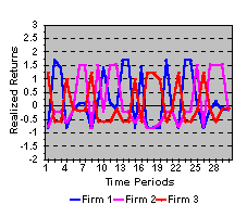
You start by explaining your investment objectives; in response the statistician brings up on a computer screen the graph in Figure 1.4.

The data in the graph gives you some insights into your investment problem.

First, the average return provides a measure of the return that you can expect to receive from a stock.

Second, the returns on the individual stocks appear to be highly volatile, and thus a significant amount of your personal wealth could easily be lost. This volatility can be measured by either the variance or the standard deviation of the returns.

Third, the returns from firms 1 and 2 tend, to some degree, to move together, while the return from Firm 3 appears to be counter-cyclical. Such co-movement is measured by the covariance of returns, and you can control your exposure to these very volatile returns by spreading your wealth among the three firms instead of investing in any one firm.

You explain that your investment decision has an investment horizon of one period starting from now. As a result, you are really only concerned with future returns but the sample provided by the statistician consists of past returns. Why is this relevant to your decision problem?

The statistician explains that we can view past returns as forming an independent random sample drawn from some underlying distribution of possible returns (called the population distribution). In the course of this conversation you find that the statistician uses some unfamiliar terms that have technical meanings. However, you will learn about the definition and properties of these terms when you study Chapter 2 on Population Statistics.

The statistician explains that from past return data, you can construct sample estimates of important parameters of the underlying distribution. This is in contrast to the financial analyst, who attempts to estimate the population distribution directly. If the population distribution does not change over time, then the sample estimates of the mean, variance and covariance will have nice sample properties, such as unbiasedness and consistency.

The statistician noted that the returns appeared to be independent over time. That is, future returns could not be predicted from past patterns of returns. This led to discussion of the concept of market efficiency because this observation was consistent with the weak form of the efficient markets hypothesis. Accordingly, powerful statistical results such as the central limit theorem can be applied to estimate the distribution of expected returns.

The statistician's work yields some sample estimates of the expected returns, variances, and covariances:

You can learn how these are computed in the topic Sample Statistics in Chapter 2. Chapter 2, Portfolio Statistics, helps you understand the relationship between observed samples and sample estimates of returns and variances.

(C) Copyright 1999, OS Financial Trading System