Chapter 4 on Markowitz Diversification showed you how to calculate the optimal portfolio weights for a target expected return and then to depict the solution graphically by plotting risk and return. In this chapter we describe the relationship between portfolio weights and the associated risk and return. This geometric analysis was first provided by Markowitz (1952).

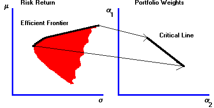
Note that each portfolio results in a single portfolio point in risk/return space. In fact, each point on the frontier corresponds to some set of portfolio weights. As a result, associated with the efficient frontier defined over risk and return is an equivalent "frontier" defined over portfolio weights. This "frontier" is called the critical line.

This association is illustrated in Figure 5.1 for the case of three securities.

In this chapter we characterize the critical line from the geometry of the three-firm problem. The CAPM Tutor subject Geometric Derivation, helps you gain a visual understanding of the portfolio problem. You should choose this subject to accompany this chapter. Clicking on the Frontier button in CAPM Tutor displays the minimum-variance frontier for the Three-Firm Case. You can choose different portfolios by clicking on different parts of the minimum-variance frontier. This allows you to observe the construction of, and movement along, the critical line depicted in Figure 5.1.

Our starting point is the now familiar set of expected returns and the variance/covariance of returns. We construct the optimal portfolio weights in several stages.

First, we reduce the problem from a three-dimensional one (i.e., solving for portfolio weights for securities 1, 2, and 3) to a two-dimensional one. We do this by observing that, given that the weights for securities 1, 2, and 3 sum to 1, once we know the weights of 1 and 2, we know the weight of 3. The portfolio weights that provide a target expected return form a straight line called the isomean line.

Making the same reduction, we can also calculate the portfolio weights that all have the same variance. Geometrically it turns out that these portfolios form an ellipse, called the isovariance ellipse.

These two topics are combined to obtain the critical line. Every point on the critical line is a point of tangency between an isomean line and an isovariance ellipse. Construction of the critical line proceeds by finding two points that lie on it. The first is the global minimum-variance portfolio and the second is a tangency point. Finally, the critical line is identified in the topic Construction of the Critical Line.

(C) Copyright 1999, OS Financial Trading System