A mathematically tractable approach to solving the portfolio problem is to build the constraints directly into the objective function by introducing Lagrange multipliers. The first constraint,

is built into the objective function,

using a Lagrange multiplier. This multiplier is a number, that equals:

It is the "marginal variance" of the target expected return. It measures how much additional portfolio risk an investor must assume to attain a slightly bigger target return.

The second Lagrange multiplier is a little more difficult to interpret because the exogenous variable is the requirement that the portfolio weights sum to one.

The Lagrange objective function for the risk minimization problem with the desired return constraint is:

Since each constraint is an equality constraint, the minimum risk portfolio is found by setting the first-order conditions to zero

for all i securities and the multiplier j equal to 1 and 2. The second-order conditions, which ensure that we are at a minimum, are satisfied since the variance is a convex function of the portfolio weights.

The first-order conditions define a system of equations that are linear in portfolio weights and Lagrange multipliers. Therefore, they can be conveniently solved by matrix techniques. CAPM Tutor solves this problem for the default data set or for your own data sets.

It is convenient to consider the three-firm form of the general problem first because it is easy to generalize from the solution to this smaller problem to get the solution to the general N-security problem. The objective function for the three-firm problem is:

The first-order conditions are:

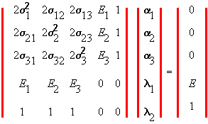
It is useful, first, to express this system of linear equations, and then solve it, in matrix form. In this form we separate out the following variables. The endogenous variables are the alphas (portfolio weights) and the two Lagrange multipliers. The exogenous variables are the set of expected returns for each security and the variance/covariance matrix of returns. Rewritten in matrix form, the first-order conditions are:

Now denote the "risk/return" matrix on the left-hand side of the above as V, the vector of endogenous portfolio weights/Lagrange multipliers by A, and the vector on the right-hand side by W. Our objective is to solve for A from the system of equations represented as:

VA = W.

The solution to the three-firm problem is obtained by inverting V and pre-multiplying both sides by this inverse:

The beauty of the matrix approach is that it reveals the structure of the solution. The solution to the N-security problem takes exactly the same form as the three-firm problem, except that the matrix is larger.

Therefore by inverting the risk/return matrix, the solution for the general case is also given by

This solution provides the optimal (minimum-variance) portfolio weights for the general N-security problem (which has (N+2)X(N+2) linear equations and N+2 unknowns) when the desired return equals E. By varying the desired return, E, the entire efficient frontier can be traced out. Note that the once the inverse of the matrix is computed, the equation for the efficient frontier as a function of E can be determined using only the last two columns of V because the first three rows of W are zero for the three-firm case. Similarly, the first N rows of W are zero for the N-security case.

To make the N-security case more concrete, let us explore the structure of the above matrixes in a little more detail. First, consider the V matrix in Table 4.2. This consists of a submatrix that is 2 times the variance/covariance matrix of the N-security returns. This submatrix is then augmented (i.e., an additional set of two rows/columns are added). The first row/column is the expected return vector with two zeros added, and the second row/column consists of 1's with two zeros added. For the general NxN case, this same structure is maintained. That is, the twice the NxN variance-covariance matrix is the sub-matrix and the augmented matrix is the expected returns for the N securities and 1's with the last two components being zero.

In Table 4.2 the A vector contains the N portfolio weights and the two Lagrange multipliers. The W vector is all zero except for the last two elements.

The above solution is applied in topic 4.9, titled the Three-Firm Case: Application of Mean Variance Theory.

(C) Copyright 1999, OS Financial Trading System