4

4.3 INVESTMENT OPPORTUNITY SET

In the portfolio selection problem, detailed in topic 4.2, you have seen that it is useful to be armed with the basic information:

1. The expected return for each security.

2. The variance of the expected return for each security.

3. The covariance of returns for each pair of securities.

How you get this information depends upon the statistical approach that you have taken. These estimates could either be direct estimates of the population statistics (for example, the financial analyst approach) or more likely sample statistics of the population using a database of historic returns.

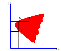
Given this basic information, it is possible to calculate the expected return and standard deviation for any portfolio. If you do this for a very large number of portfolio weights, and plot each calculation as a point in expected return/standard deviation space, you would get a scatter plot that looks like figure 4.1.

Figure 4.1

Investment Opportunity Set

All points fall within the heavily shaded region. You can see this fact by applying CAPM Tutor to the default data set, that can produce the scatter plot for the Three-Firm Case. The shaded area is called the investment opportunity set. It shows you all possible risk and return combinations that are available in the market.

An investor who wants to squeeze every bit of performance out of a portfolio would pick only certain points in the shaded area. Such an investor would want a portfolio that maximizes the expected return for a given level of risk, or minimizes the standard deviation for a target level of return.

For example, consider portfolios A and B above. Both portfolios have the same portfolio standard deviation but portfolio A has a higher expected return. Therefore, portfolio A dominates portfolio B. Similarly, portfolio A dominates portfolio C because both have the same expected return, but C has a larger portfolio standard deviation.

In summary, a portfolio dominates a set of other portfolios in risk and return space if either of the following two cases is satisfied:

1. For a given expected return, all other portfolios have a larger standard deviation.

2. For a given standard deviation, all other portfolios have a smaller expected return.

An investor who is interested in optimizing portfolio performance would never choose a dominated portfolio. Using CAPM Tutor you might want to see this for yourself by constructing some portfolios that dominate the equally weighted, naively diversified, portfolio for the Three-Firm Case. Then, you can check whether an optimizing investor would make different investment decisions than would the naive investor for this problem.

The boundary of the shaded area in Figure 4.1 is called the minimum-variance frontier because it represents portfolios that have the smallest variance (or standard deviation) for a given level of expected return.

Next we will characterize the part of the minimum-variance frontier that is of interest to investors in the topic The Efficient Frontier.

previous topic

next topic