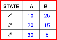
Assume there are two stocks, A and B. There are three states, s1, s2, and s3. Each state has an equal chance of occurring, and the value of the stocks in each state is Table 2-2:

Expected values of the two stocks are given by

E(A) = 10/3 + 20/3 + 30/3 = 20

E(B) = 25/3 + 15/3 + 5/3 = 15

The variances and the covariance are given by

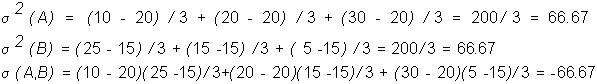
A portfolio consisting of +1 shares of stock A and +1 shares of stock B has an expected payoff of 35 and a variance of zero.

Suppose the price of A is 18.182, and the price of B is 13.636. Then the expected return from each stock is computed as follows:

E(RET(A)) = (1/3)[(10-18.182)/18.182 +(20-18.182)/18.182+(30-18.182)/18.182]

E(RET(B)) = (1/3)[(25-13.636)/13.636 +(15-13.636)/13.636+(5-13.636)/13.636]

At these prices, both expected returns are approximately 10%.

It is easiest to compute the portfolio variance using the matrix multiplication method. The last term, raised to the power T, denotes the transpose of the vector of portfolio weights. This merely denotes that the portfolio weights are stacked vertically (i.e., form a matrix with 1 column and N rows) in the matrix multiplication procedure.

That is, the variance-covariance matrix of returns is pre-multiplied by the vector of portfolio weights. This product is post-multiplied by the portfolio weight vector. This is the product of three matrixes (1xN)(NxN)(Nx1) assuming that there are N risky financial securities in the economy, which results in a 1X1 matrix (i.e., number) equal to the portfolio variance.

Recall that the Three-Firm Case has the population parameters in Table 2.3:

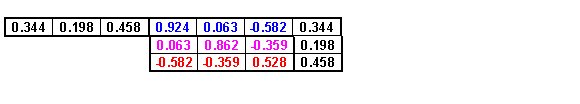
Suppose you want to form portfolio A so that the E(Return) = 0.13 when the weights are:

Security 1 = 0.344, Security 2 = 0.198, Security 3 = 0.458.

E(Return A) = (0.344)(0.229) + (0.198)(0.138) + (0.458)(0.052) = 0.13

The portfolio standard deviation is computed from the variance-covariance matrix of returns:

For the Three-Firm Case, the variance-covariance matrix of returns for firms 1,2, and 3 is:

The diagonal terms are variances. That is, .924 is the variance of returns for Firm 1, .862 is the variance of returns for Firm 2 and .528 is the variance of returns for Firm 3. The off diagonal terms are the covariances. For example, -.582 is the covariance of the return of Firm 1 and Firm 3.

The easiest means for computing the portfolio variance is to apply matrix multiplication methods. Let the portfolio weights be depicted in black. Then, by pre- and post-multiplying the transpose of the weight vector, the portfolio variance is:

This yields a portfolio variance of 0.075, and thus the portfolio standard deviation is 0.274.

(C) Copyright 1999, OS Financial Trading System